Apache Logs

25 Aug 2016

The idea of this post is to try to make an analysis of the raw data (logs) in the Common Log Format to visualize some interesting details like traffic trends, status and more! It is true that we can always have automated tools such as a SIEM and / or SOAR that can do this job much more optimally, but it is always good to know how it can be done otherwise.

The first thing to do is to load the necessary libraries

• library(readr)
• library(rgeolocate)
• library(dplyr)
• library(IPtoCountry)
• library(lubridate)
• library(ggplot2)

Once we have the necessary packages to work our data we will proceed to read the raw file (csv, raw, etc..)

In my case it is called (“access.log”)

logs <- read_log("access.log", skip=0, col_names=FALSE)

Once we store the data in a variable called “logs”, it is important to see and know the structure and the name of the columns in order to start manipulating it in a simple and efficient way

colnames(logs)
[1] "X1"  "X2"  "X3"  "X4"  "X5"  "X6"  "X7"  "X8"  "X9"  "X10"

We can select the “column” data we will need later.

final <- logs[,c('X1','X4','X5','X6','X7','X8','X9')]

Now that we are able to inspect the data and know what information each column has, we will rename them to be more friendly.

filtrado <- setNames(final, c("ip_address", "date_time", "to_url","http_status","client_size","URL", "User-agent"))

At the moment I will create an additional column to use a function called IP_country that will simply allow us to reference an ip to a country.

city <-mutate(.data = filtrado,country = IP_country(ip_address))

What we will do next is to set the format of the data in the column that has the date, as follows:

Currently the column date_time is as a character type, so we will use POSIXct

class(city$date_time)

Now there are several ways to do this:

If we have something like this 03/Mar/2016:18:22:16 in the date_time we can use:

as.POSIXct(gsub('Mar','03',city$date_time))  

Or use a specific format :)

as.POSIXct(strptime(city2$date_time,"%d/%m/%Y:%H:%M:%S"))

In my case, I decided to do it this way:

city2$date_time <-(gsub('Mar','03',city$date_time))

city2$date_time = as.POSIXct(strptime(city2$date_time,"%d/%m/%Y"))

Now let’s see some analysis and what results we could get

table(city2$http_status)
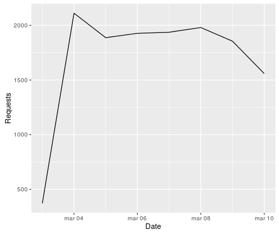
reqs=as.data.frame(table(city2$date_time))
n=23

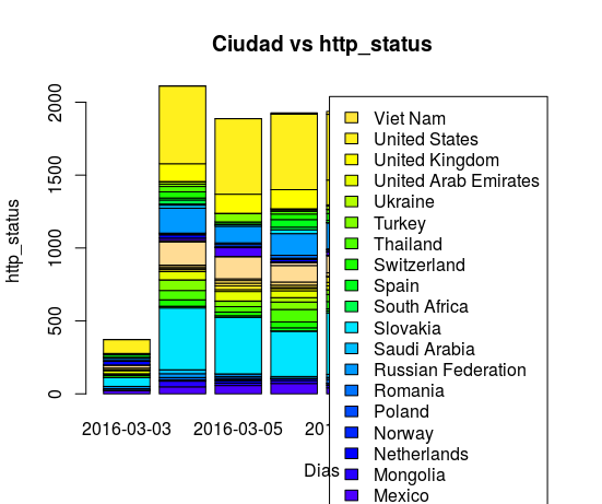
counts <- table(city2$country, city2$date_time)
barplot(counts, main="Ciudad vs http_status",xlab="Dias",ylab = "http_status", col=c(topo.colors(n)),legend = rownames(counts)) 

HTTP-STATUS

ggplot(data=reqs, aes(x=as.Date(Var1), y=Freq), title('trafico del sistio')) + geom_line() + xlab('Date') + ylab('Requests')

REQUEST

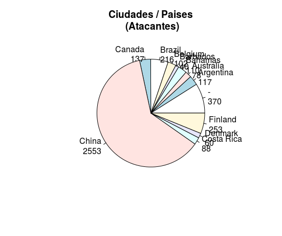
Number of attacks per city/country

mytable <- table(city2$country)
lbls <- paste(names(mytable), "\n", mytable, sep="")
pie(mytable[1:10], labels = lbls,
    main="Ciudades / Países\n (Nº ataques)")

HACKED!