A realistic cyber defense data set (CSE-CIC-IDS2018)
This dataset is the result of a collaborative project between the Communications Security Establishment (CSE) and the Canadian Institute for Cybersecurity (CIC) that uses the notion of profiles to generate a cybersecurity dataset in a systematic way. It includes a detailed description of intrusions along with abstract distribution models for lower level applications, protocols or network entities. The dataset includes seven different attack scenarios, namely brute force, botnet, denial of service, web attacks and network infiltration from within. For more information on the creation of this dataset, see this article by researchers from the Canadian Institute for Cybersecurity (CIC) and the University of New Brunswick (UNB): Towards the Generation of a New Intrusion Detection and Intrusion Traffic Characterization Dataset.
Info: Data
NOTE: For the following examples only a sample of the entire DataSet was used.
We configure the work area and load libraries
rm(list = ls())
setwd("/home/gelvis.rodriguez/Desktop/")
library(ggplot2)
library(tidyverse)
library(plotly)
Now we load the information:
datos <- read.csv("ips.csv", stringsAsFactors = FALSE)
We verify the structure it has:
> head(datos)
        Attacker        Victim      Attack.Name             Date Attack.Start.Time Attack.Finish.Time
1   18.221.219.4 18.217.21.148   FTP-BruteForce   Wed-14-02-2018             10:32              12:09
2    13.58.98.64 18.217.21.148   SSH-Bruteforce   Wed-14-02-2018             14:01              15:31
3 18.219.211.138 18.217.21.148    DoS-GoldenEye Thurs-15-02-2018              9:26              10:09
4 18.217.165.70) 18.217.21.148    DoS-Slowloris Thurs-15-02-2018             10:59              11:40
5   13.59.126.31 18.217.21.148 DoS-SlowHTTPTest   Fri-16-02-2018             10:12              11:08
6  18.219.193.20 18.217.21.148         DoS-Hulk   Fri-16-02-2018             13:45              14:19
Now we will proceed to generate our graphics data to better understand the information.
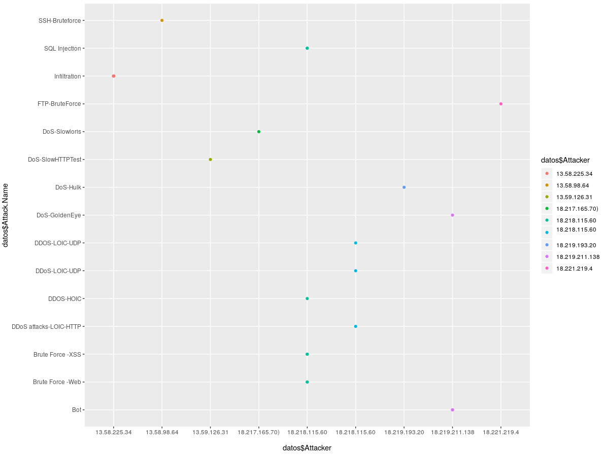
Attacking IP with your Attack Type.
ggplot(datos = datos, mapping = aes(x = datos$Attacker, y = datos$Attack.Name)) + geom_point(aes(color = datos$Attacker))
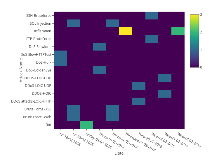
Type of Attack and Date Detected.
p  <- plot_ly(data = datos, x = ~Date, y = ~Attack.Name)
p
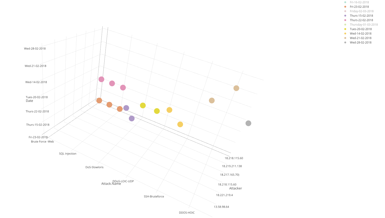
Type of Attack, Date Detected and Attacker’s IP (3D and interactive).
plot_ly(datos, x = ~Attacker, y = ~Attack.Name, z = ~Date) %>%
  add_markers(color = ~Date)
We could also obtain the geographic location of each IP of the attackers, but in other posts we have already done that.